 | 02 May 2018
An approach for the estimation of the aggregated photovoltaic power generated in several European countries from meteorological data
Yves-Marie Saint-Drenan
Lucien Wald
Thierry Ranchin
Laurent Dubus
Alberto Troccoli
Classical approaches to the calculation of the photovoltaic (PV) power generated in a region from meteorological data require the knowledge of the detailed characteristics of the plants, which are most often not publicly available. An approach is proposed with the objective to obtain the best possible assessment of power generated in any region without having to collect detailed information on PV plants. The proposed approach is based on a model of PV plant coupled with a statistical distribution of the prominent characteristics of the configuration of the plant and is tested over Europe. The generated PV power is first calculated for each of the plant configurations frequently found in a given region and then aggregated taking into account the probability of occurrence of each configuration. A statistical distribution has been constructed from detailed information obtained for several thousands of PV plants representing approximately 2 % of the total number of PV plants in Germany and was then adapted to other European countries by taking into account changes in the optimal PV tilt angle as a function of the latitude and meteorological conditions. The model has been run with bias-adjusted ERA-interim data as meteorological inputs. The results have been compared to estimates of the total PV power generated in two countries: France and Germany, as provided by the corresponding transmission system operators. Relative RMSE of 4.2 and 3.8 % and relative biases of −2.4 and 0.1 % were found with three-hourly data for France and Germany. A validation against estimates of the country-wide PV-power generation provided by the ENTSO-E for 16 European countries has also been conducted. This evaluation is made difficult by the uncertainty on the installed capacity corresponding to the ENTSO-E data but it nevertheless allows demonstrating that the model output and TSO data are highly correlated in most countries. Given the simplicity of the proposed approach these results are very encouraging. The approach is particularly suited to climatic timescales, both historical and future climates, as demonstrated here.


Time series of photovoltaic (PV) power generated within a region are needed for prospective studies on the transformation of the electricity supply system. Under classical approaches an accurate calculation of the power generated by PV plants in a region requires the knowledge of the detailed characteristics of the plants. A few cases can be found where enough information is available, and can be used for the model development and/or validation (see e.g. Jamaly et al., 2013; Lingfors and Widén, 2016; Shaker et al., 2015, 2016). Plant production data are however most often unavailable to the public. They may be collected from e.g. the operators of PV plants but this represents a huge amount of work. Hence, an accurate calculation of the PV power generated in any European region with a classical method represents an exhaustive and time-consuming task and is intractable. Alternatively, statistical approaches may be used to train models from historical time series of the aggregated PV generated power, such as those published by the transmission system operators. In this case, the collection, understanding and quality check of the training data is primordial to ensure accurate model output. Though more practical than the classical approaches, these statistical approaches are also time consuming because of the handling of the data and they cannot be applied in regions where no training data is available. Another common practice consists in estimating the total power generated in a region by upscaling the power generated by a subset of reference plants (Schierenbeck et al., 2010; Lorenz and Heinemann, 2012; Shaker et al., 2015, 2016; Saint-Drenan et al., 2016; Bright et al., 2017; Pierro et al., 2017; Killinger et al., 2017). The major obstacles to this practice is on the one hand the establishment of criteria on the selection of the plants that are statistically representative of the region and their number, and on the other hand, the access to measurements of the selected plants. In addition, those methods only allow estimating the PV power generation for historical periods where measurements are available, and their extrapolation to other periods is not straightforward. This can be a major drawback for e.g. generation adequacy study or prospective analysis where scenarios with long time series are needed. A further option consists in selecting a simple PV model, with a very limited number of unknowns (Jerez et al., 2015), whose implementation for any region is easy to do at the expense of the model accuracy. Finally, several authors propose to consider a mix of different key parameters, where the distributions are chosen by the authors (Marinelli et al., 2015; Schubert, 2012). This requires a deep expertise of the domain. This approach is limited to a few regions and cannot be used to model all EU countries.
This brief survey of the proposed approaches demonstrates the need for a new approach that offers a better trade-off between implementation constraints and model output accuracy. This paper describes a method addressing this need. It has been developed in the framework of the EU-funded Copernicus Climate Change Service ECEM1 (European Climate Energy Mixes) project which aims at producing, in close collaboration with prospective users, a proof-of-concept climate service, or demonstrator, whose purpose is to enable the energy industry and policy makers to assess how well different energy supply mixes in Europe will meet demand, over different time horizons (from seasonal to long-term decadal planning), focusing on the role climate has on the mixes (Troccoli et al., 2017).
The innovation of our method is the extension of the regional PV model proposed by Saint-Drenan (2015) and Saint-Drenan et al. (2017) to any region, without the need for a priori knowledge of the characteristics of the installed PV plants. To this end, the plant-related parameters which are needed as input to the PV model are expressed as a function of known solar resource characteristics, making thus the model generalizable to any region, namely beyond Germany where the approach was originally tested. This is achieved in two steps: firstly, by reducing the number of inputs to the PV model by the means of an analytical function for the statistical distribution of the module orientation and, secondly, by expressing the parameters of the chosen analytical functions as a function of known geographically-dependent information (optimal tilt angle).
The paper is organized as follows. After a short summary of the regional PV model proposed by Saint-Drenan (2015) and Saint-Drenan et al. (2017) in Sect. 2.1, the reduction of the number of parameters achieved by the use of an analytical function is detailed in Sect. 2.2. The approach chosen to relate the parameters of the analytical function to known geographically-dependent quantities is then explained in Sect. 2.3. Implementation details are provided in Sect. 2.4. The results of a validation of the model are described in Sect. 3, where the model output has been compared to estimates of the total PV power generation of France and Germany provided by transmission system operators (TSOs). Finally, the results and potential improvements of the approach presented are discussed in Sect. 4.
Our approach for modelling the PV power generation in any country use a generic PV model which needs only the distribution of the two module orientation angles as inputs. This model is introduced in Sect. 2.1 and the methodology for estimating the distribution of the module orientation angles in any location is described in the Sect. 2.2 and 2.3. Finally, some implementation details are given in Sect. 2.4.
2.1 Description of the model for the aggregated PV power produced in a region
The proposed method is built upon previous works by Saint-Drenan (2015) and Saint-Drenan et al. (2017), where a model for the aggregated PV power produced by a fleet of PV plants installed in a region is described. The authors have showed that an accurate estimate of the German PV power generation can be obtained by using the statistical distribution of the orientation angle of PV panels as the sole plant-relevant input to the model (Fig. 1). The model is based on the simple idea that the aggregated PV power generated in a region is the sum of the normalized outputs of all plants with characteristics Ai multiplied by the proportion wi of plants having the characteristics Ai in the whole set of plants installed in the considered region. The regional PV power generation can therefore be expressed as follows:
Where PPV(x,t) is an estimate of the aggregated power produced by all PV plants located at x at time t [W W], G(x,t) is the global horizontal irradiance (GHI) received at x and t [W m−2], Ta (x,t) is the air temperature at x and t [∘C], fPV(…) is a function representing the single PV plant model used to calculate the normalized PV power [W W].
A first advantage of the chosen regional PV model is that each important configuration is considered only once and the number of configurations Ai can be optimized in order to limit the calculation costs. A second advantage is the high flexibility offered by the use of an analytical function to describe the statistical distribution of the characteristics of the plants installed in a region.
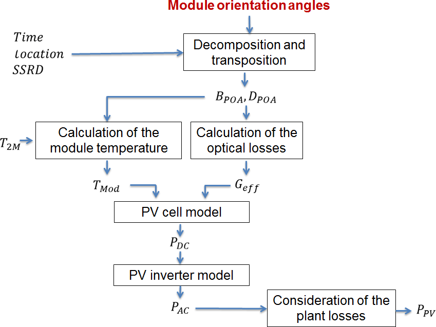
The function fPV in Eq. (1) represents a single plant model, which needs to be chosen prior to the implementation of the proposed approach. In Saint-Drenan (2015) and Saint-Drenan et al. (2017), the authors demonstrated that a simple model with a limited number of input parameters yields good results for regional application. With the chosen model, the set of characteristics Ai is only composed of the module tilt angle γ and azimuth angle α or orientation. The Ai's, which are a function of (α, γ), are hereafter referred to as reference configurations. There are two steps for the implementation of the regional PV model that are described in the following section: the estimation of the weights wi and the choice of the reference configurations. A detailed description of the chosen model which is illustrated in Fig. 1 can be found in e.g. (Saint-Drenan, 2015).
2.2 Modelling the weights wi
Saint-Drenan (2015) and Saint-Drenan et al. (2017) have created a dataset of peak power and module orientation angles for 35 000 PV plants located in Germany, which is used here. This amount of plants represents approximately 2 % of the number of plants installed in Germany. It is assumed that this dataset is representative of all plants in Germany. A realistic example of the relationship between wi and Ai at country level may be derived from this dataset. Figure 2 exhibits the share wi of installed capacity per module orientation evaluated from this dataset. One may note the high share of installed capacity for modules with a tilt of 20∘ southwards facing (orientation 180∘).

Figure 2Share of the installed capacity per module orientation evaluated from the 35 000 PV plants installed in Germany (coloured squares). Black squares denote the set of 19 reference orientations used for the implementation of the regional model.
The use of Eq. (1) requires that the space spanned by α and γ is properly sampled in order to obtain a robust estimation of the plant shares wi corresponding to the sampled orientations in that equation. The smoothness and form of the joint distribution displayed in Fig. 2 suggest that it may be possible to fit an analytical relationship, therefore reducing the number of parameters used to describe it. We propose to use the product of two Gaussian distributions:
In Eq. (2), the first product term corresponds to the normal distribution of α, characterised by a mean value μα and a standard deviation σα. The second product term corresponds to the normal distribution of γ, characterised by a mean value μγ and a standard deviation σγ. It appears reasonable to assume that the distribution of α is centred on a southwards orientation, so that μα can be set to 180∘. In Eq. (2), it is assumed that the distributions of the α and γ are independent – from Fig. 2 this assumption is an acceptable first-order approximation. A different notation has been used for the weights wi in Eqs. (1) and (2) since, as further explained in Sect. 5, values calculated with Eq. (2) must be normalized before being inserted into Eq. (1).
The use of the analytic form in Eq. (2) for the weights allows reducing the number of plant-relevant parameters down to three, which are the mean and standard deviation of γ and the standard deviation of α. This reduced form has been tested using the German solar plants. We found an average value of 20.6∘ for μγ and values of 19.3 and 10.8∘ for σα and σγ. The empirical histograms of the tilt and azimuth angles are compared to their fitted normal distributions in Fig. 3. The match between the histograms is not perfect but it seems an acceptable first-order approximation.
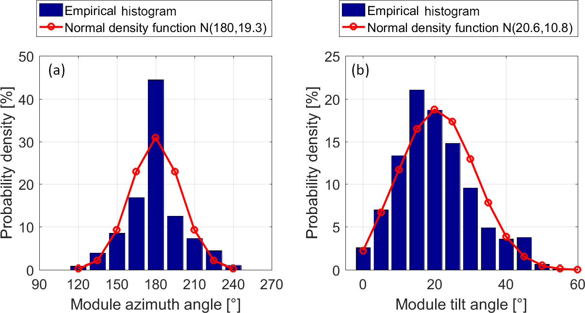
Figure 3Comparison of the experimental histograms of two module orientation angles (blue bars) with the fitted normal distribution function (red lines) for the module azimuth angle (a) and the module tilt angle (b). N(180, 19.3) (a) means that the average orientation is 180∘ and the standard deviation is 19.3∘. N(20.6, 10.8) (b) means an average tilt angle of 20.6∘ and a standard deviation of 10.8∘.
2.3 Parameterisation of the relationship between the distribution of the orientation of PV modules and the geographical location
The three plant-related parameters necessary to calculate the total PV power produced in a given region from meteorological data has been determined above in the specific case of Germany. How can these three parameters be extended to other countries/regions? At this stage, one possibility may consist in using ones own expertise on the characteristics of PV plants installed in the considered regions as in Marinelli et al. (2015); Schubert (2012); another is a detailed statistical analysis of a dataset of plant information installed in the studied areas. Both ways hamper the easy use of the regional model aimed at in this work. To address this issue a parameterization of the three parameters is proposed in this section, which makes the model implementable in any region without any prior knowledge on the installed PV plants.
The statistical distribution of the plant capacity as a function of the module orientation of a region is the result of individual choices on the configurations of each single plant. It is affected by many factors of different nature such as the characteristics of the solar resource, the shading profile, architectural characteristics, different installation practices, etc. All these factors cannot be taken into consideration and we make the assumption that the most important one is the characteristics of the solar resource. We propose to take this into consideration through the use of an optimal tilt angle. The optimal tilt angle corresponds to the value of the tilt angle of a southwards oriented module yielding the largest annual output. In this work, we use the raster file of optimal tilt angles available on the PV-GIS website (http://re.jrc.ec.europa.eu/pvgis/), which is displayed in Fig. 4a as our starting point.
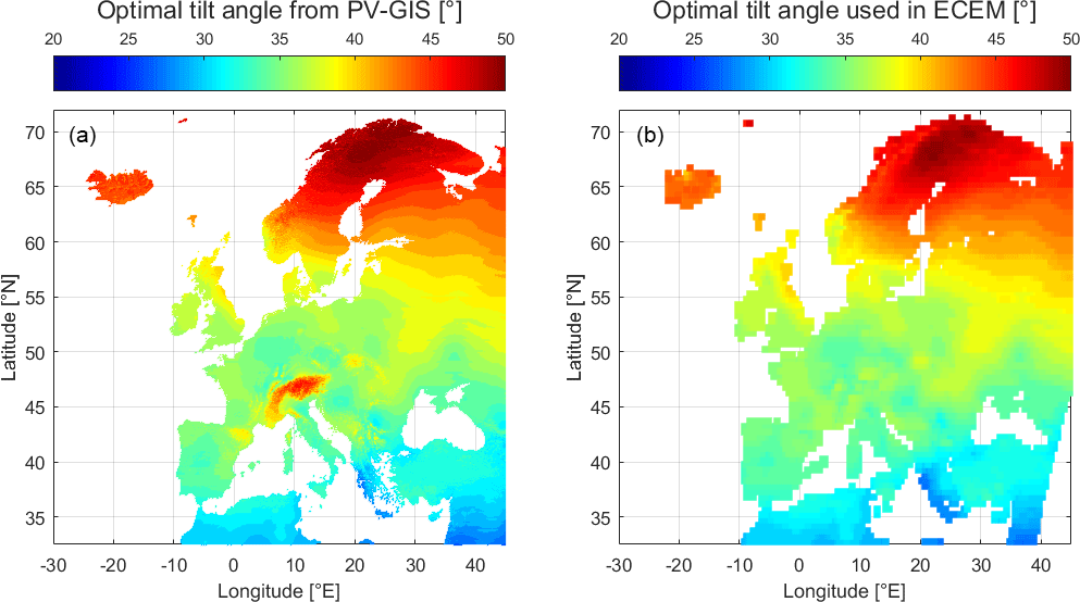
Figure 4(a) Optimal tilt angles taken from the PV-GIS website (http://re.jrc.ec.europa.eu/pvgis/). (b) Optimal tilt angles used for the present work where high values present in mountainous regions have been filtered out.
It can be observed in Fig. 4 that the optimal tilt angle γopt is ranging between 30 and 35∘ in Germany while the average value for the tilt angle has been found equal to 20.6∘ in the previous section. The reason for this mismatch is that a tilt angle smaller than the optimal tilt angle is commonly used to install more PV capacity per unit of surface and maximize the economic output of the plant. This practice has become more frequent with decreasing PV price and scarce available surfaces for new installations. We propose to quantify the mismatch between these two angles by a coefficient f. The average tilt angle μγ can thus be expressed as
The unknown factor f can vary from one plant to another since it depends on numerous factors such as the solar resource, the plant cost per peak capacity or the land price. It may thus exhibit spatial and time variation and an accurate determination of this coefficient for all European countries may be difficult. We assume that this factor is spatially constant. Considering the average value of the tilt angles, which is equal to 20.6∘, the factor f should be chosen between 0.6 (20.6/35) and 0.7 (20.6/30). Given that the chosen dataset includes an under-representative share of large solar park, that usually have an optimal tilt angle (Saint-Drenan, 2015), we have chosen the upper bound for f (f=0.7). Similarly, we assume the standard deviations of the azimuth and tilt angles spatially constant and set them to the values found with the set of PV plants installed in Germany (19.3 and 10.8∘ for the azimuth and tilt angle).
The weights corresponding to the different orientation angles are finally estimated using Eq. (2), where the mean tilt angle is taken equal to the optimal tilt angle time the factor f=0.7 and the standard deviations of the azimuth and tilt angles are considered constant and equal to 19.3 and 10.8∘ respectively.
2.4 Implementation details
Some implementation details have been intentionally omitted in the previous sections for the sake of clarity and conciseness. This section provides some important details for the implementation of our method.
For the implementation of Eq. (1), the identification of a limited number of vectors Ai describing the reference module orientations is necessary. The accuracy of the model output and the computation cost will depend on the number of vectors chosen. It is thus an important step for an efficient use of our model. We used a set of 19 module orientation angles: three azimuth angles (170, 180 and 190∘) and 7 tilt angles ranging from 0 to 60∘ with a step of 10∘. These are represented by black squares in Fig. 2.
Our parameterization of the distribution of the module orientation is a function of the optimal tilt angle found on the PV-GIS website. This dataset is displayed in the left map of Fig. 4, where it can be observed that greater than average values are present in mountains (see e.g. regions of the Alps or the Pyrenees). These high values are presumably stemming from the high irradiation values present at high elevations. Since little PV plants are installed in these regions and to avoid overestimation of the tilt angle in the region neighbouring the mountains, these values have been filtered out. The resulting data are displayed in the right map of Fig. 4.
As already mentioned in Sect. 3, the expression given in Eq. (2) cannot be directly used to estimate the weights wi needed by Eq. (1). Indeed, for a finite sample of orientation angles Ai, the sum of the values evaluated with Eq. (2) is not equal to unity. To address this issue, estimated with Eq. (2) is normalized as follows to yield wi:
The scalars δα and δγ in Eq. (6) represent respectively the resolutions of the azimuth and tilt angles, which are both equal to 10∘ in our implementation.

Figure 5Spatial distribution of the installed PV capacity in France and Germany for the year 2014. The installed capacity is aggregated on the pixel used for the calaculation which have a resolution of 0.5∘.
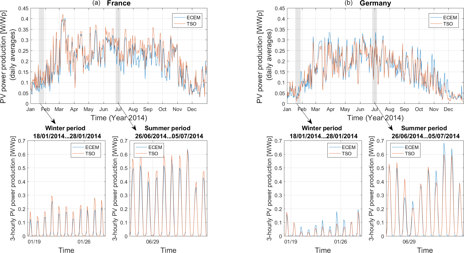
Figure 6Comparison of the model output (blue lines) with TSO estimates (red lines) of the PV power generated in France (a) and Germany (b). The data are displayed over the year with a daily time resolution in the two plots above and for two example weeks in a 3-hourly time resolution in the two lower plots.
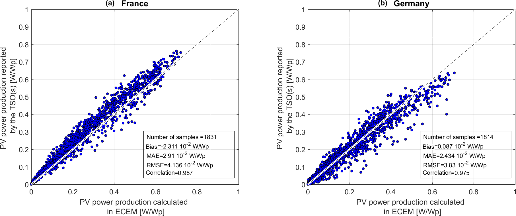
Figure 7Scatter plots of the TSO data against model outputs for France (a) and Germany (b) for the calculation based on the spatially resolved installed capacity of the year 2014.
3.1 Evaluation methodology
The model has been assessed by comparing its outputs to the PV power generated within a country. Given the approach is influenced by uncertainties in the input meteorological parameters, this comparison allows only an indirect evaluation of our model and not a quantification of the modelling accuracy. However, this approach offers a good balance between accuracy and versatility. The goal of this evaluation is thus to verify the plausibility of the model output for a particular model set up. Not only is there a lack of certainty in the input meteorological data but also there are various sources of uncertainty impacting the TSO data as well as the installed capacity used by the model, both making the conclusion of the validation difficult. To address these issues, we conduct the validation in two steps. In the first step, the validation is conducted for two countries: France and Germany, where we have long experience with both the installed capacity and the TSO data. In this first step, the impact of the uncertainty on the installed capacities and TSO estimates is under control but its spatial extension is limited. We therefore conduct a second step, where TSO data from 16 countries are considered. Given the lack of available information on the installed PV capacity in these countries, it is assumed spatially and temporally constant. The actual installed capacity being unknown, the validation is made by evaluating the correlation coefficient between TSO data and model output.
3.2 Detailed evaluation of the model output for France and Germany
The assessment is first performed for Germany and France for the year 2014. The choice of these two countries has been strongly motivated by the comparatively high level of knowledge of their electricity supply structure and the availability of the data to conduct the validation. The PV power data was provided by the TSOs themselves with a time resolution ranging from 15 min to 1 h. A visual analysis of the time series was performed to control the data. The data was aggregated into 3 h means to conform to the temporal resolution of the meteorological data. Instants with no production by PV (night time) were excluded from the comparison.
The German case is used to validate the assumption made that the statistical quantities evaluated with 35 000 plants can be generalized to the ca. 1 500 000 plants installed in Germany at that time. France has a different level of PV development compared to Germany and is located at slightly different latitudes. This second case will test the validity of our approach to generalize the statistical quantities evaluated in Germany to another country with somewhat different meteorological conditions.
Gridded values of the normalized PV power were computed with the model using the bias-adjusted ERA-interim data proposed by the ECEM project (Jones et al., 2017) as meteorological inputs. A bias-adjusted dataset was preferred to the original ERA-Interim re-analysis dataset in order to limit the effect of error in the input meteorological data on the assessment of model performance. The bias-adjusted ERA-Interim covers the period from 1 January 1979 to 31 December 2016 and is covering Europe with a spatial resolution of 0.5∘ × 0.5∘. The domain covered by the data extends between 21.75 and 45.25∘ in longitude and between 26.75 and 72.25∘ in latitude. The two meteorological variables used for the calculation were the solar surface radiation downward (SSRD, also known as GHI) and air temperature at 2 m. As the input meteorological data has a time resolution of 3 h for SSRD and 6 h for temperature, an increase of the time resolution was needed to properly estimate the PV power generation with respect to the variation of the sun position with time. For this purpose, the temperature and clearness index (the ratio of SSRD to the irradiation at the top of atmosphere) were resampled down to a time resolution of 5 min by a linear interpolation technique. The normalized PV power was calculated with these resampled inputs and then summed up on 3 h periods, which is the original time resolution of the solar radiation data.

Figure 8Histograms of the ratio of actual plant tilt angles with the corresponding optimal value for different classes of nominal capacity (coloured lines). In the upper plot, the German case is calculated with the IWES database. The French case is displayed in the lower plot where data from BDPV are used.
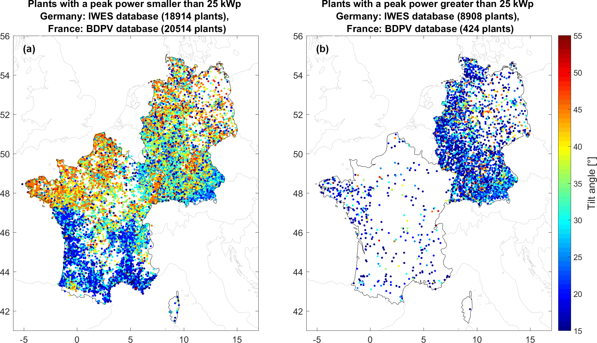
Figure 9Spatial distribution of the tilt angle for plants smaller than 25 kWp (a) and greater than 25 kWp.
By using gridded maps of the installed PV capacity in each country (Fig. 5), the generated PV power was computed at each grid cell and then spatially summed to yield the production for each country. The data on the installed PV plants used for this purpose have been retrieved from the websites of the four German TSOs (PV-DE 2014) and from a data portal of the French government (PV-FR 2014). Finally, all time series have been normalized by the total installed PV capacity, which is equal to 6.17 and 36.87 GWp for France and Germany, respectively, in 2014 (PV-DE, 2014; PV-FR, 2014). Figure 6 exhibits the time series of both measured production and model outputs for France and Germany daily and 3 h resolutions. It reveals that the seasonal variations of the PV power are well assessed by the proposed model for the two countries and that the match between model output and actual values is qualitatively good. Scatter plots of the TSO data against the model outputs are displayed in Fig. 7 for France and Germany for the 3 hourly resolution and different error metrics are also displayed in Fig. 7. The data points are well centred on the identity line for Germany while an underestimation by the model can be observed for France. These observations are confirmed by the bias, which are respectively equal to and W W for France and Germany. The correlation coefficient is large in both countries: 0.987 and 0.975 respectively for France and Germany. The MAE is respectively and W W; the RMSE is respectively and W W.
Some efforts were made to understand the reasons for the greater bias value observed for France. During this investigation we obtained access to the content of the bdpv.fr online portal (BDPV, 2018), which contains the main information for more than 20 000 PV plants installed in France. We used this new data source to compare the characteristics of the German and French PV plants and to verify the validity of our assumption for France.
The strongest assumption made in this work is to consider that the mean tilt angle is equal to the product of the optimal tilt angle and a constant f equal to 0.7. In order to verify this assumption, the ratio between actual and optimal module tilt angle has been analysed for the two countries. The histograms of this ratio are displayed for the two countries and for different classes of nominal capacity in Fig. 8. The assumed value for the ratio f is displayed by a dashed black line in these two plots. We can observe that the assumed ratio value matches well large German plants with an installed capacity greater than 500 kWp (no information on large PV plant is available in France). Data from both countries reveal that this value is not fitting actual tilt values of medium and small plants: an optimal ratio value of 0.4–0.6 would better match plants with an installed capacity between 50 and 500 kWp and a ratio value of 0.9–1.3 would be better for plants with an installed capacity smaller than 10 kWp. It is interesting to note that the optimal ratio changes with the size of the plants in a similar way for both countries. These observations indicate, that the variation of the share of PV plants according to their size between countries can bring about a deviation from the assumed factor of 0.7. A first possible explanation for bias observed in France may thus be that the distribution of French plants according to their size is different from the German one.
It would be interesting to exploit the trend observed in Fig. 8 in our model. However, information on the size of installed PV plants is missing in most European countries so that this is unfortunately impossible. Based on these new results, one can wonder whether the choice of a value of 0.7 for the ratio between actual and optimal tilt is still relevant? Given that larger plants have more weight for the calculation of the regional PV power generation than smaller plants, we consider that our estimate is not unfounded and we decide to keep this value.
In Fig. 8, it can also be observed that for PV plants with an installed capacity smaller than 10 kWp, the range of tilt angle values taken by French plants is larger than for German plants. To understand this difference, the tilt angle values of small plants have been displayed as a function of their geographic position (Fig. 9). In this map, a very large difference in tilt angles between North and South of France can be observed. This spatial difference is much more pronounced than the spatial variation that can be expected from the optimal tilt angle. Since such a marked spatial difference is not present in Germany, it could bed a second possible explanation to the observed bias in France.
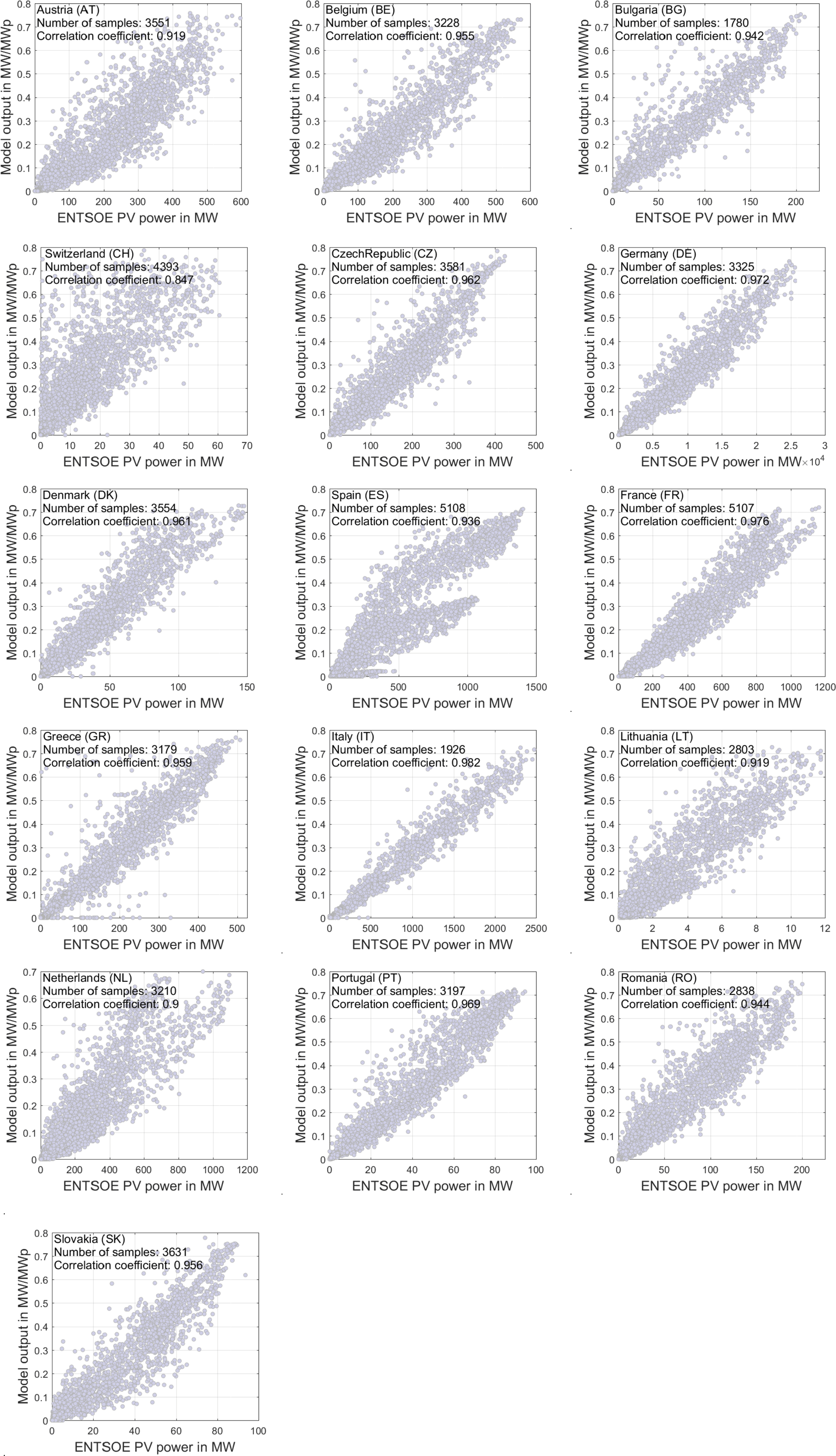
Figure 10Scatter plots of three-hourly ENTSO-E solar generation data against the corresponding model output for 16 European countries for the year 2016. The modelled PV generation has been calculated with ERA-interim data assuming a spatially constant installed capacity.
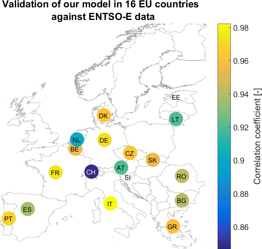
Figure 11Spatial distribution of the correlation between ENTSO-E data and model output for a three-hourly time resolution and for the year 2016.
As reported in Saint-Drenan (2015), the spatial variations of the tilt angle of small plants are resulting from regional architectural practices. It would therefore be tempting to integrate this information into our model. However, because this information is not commonly available (i.e. not even for France), it could not be accounted for in a robust way.
3.3 Model evaluation for all European countries
Though the results of this first validation can be considered as satisfactory, it is important to also demonstrate that results for Germany and France can be extrapolated to other (European) countries, also with different climates, engineering practices, etc. We therefore decided to conduct an additional validation step, in which we compared the output of our model to additional TSO data. To this end, we collected time series of solar power generation on the ENTSO-E Transparency Portal for 16 countries for the year 2015 and built 3-hourly averages to make the data comparable with the model output. The model setup is the same than in the previous validation except for the installed capacity, which is not known and thus assumed spatially and temporally constant (even in France and Germany). Indeed, the information available on the installed capacity is only updated yearly and we experiment several situations where the time series of the production were not matching with the given installed capacity (e.g. situation with production values greater than the installed capacity).
The comparison of the model output with the ENTSO-E data has been conducted for 16 countries. The scatter plot of the model output against ENTSO-E data is given in Fig. 10 for each country. As mentioned before, since the installed capacity is not known, the model output has not been scaled to the actual capacity. As a result, one should not consider the absolute error values in these plots but solely the correlation between the two time series. Accordingly, only the correlation coefficient is given in Fig. 10 and discussed in the remaining of this section. To facilitate the visualisation of the results, the correlation coefficients evaluated for the different countries are displayed as a map in Fig. 11.
With values greater than 0.97, the correlations are particularly high in Italy, France and Germany. These results confirm those obtained for France and Germany in the first validation. That the best correlation (0.982) is found for Italy is a very good surprise since no information on the PV plants installed in this country was considered in the model development. As we can see in Fig. 12, the high installed capacity in Italy (ca. 19 GWp in 2016) may account for this good performance. The correlation coefficients are high and comprised between 0.95 and 0.97 for six countries: Denmark, Belgium, Czech Republic, Slovakia, Greece and Portugal. This demonstrates that the proposed approach using the optimal tilt angle is valid at different latitudes. The low performance of the model for Spain is explained by the fact that the time series of solar generation available on the ENTSO-E website includes both photovoltaic and concentrated solar power generation. The reason for the medium performance in the remaining countries is unclear: it may stem from an intra-yearly change of the installed capacity, from lower performance of the re-analysis data in some regions or from other unidentified issues, including in the ENTSO-E generation data. It is however interesting to note that in the 16 countries, as shown in Fig. 8, the greater the installed capacity, the better the performance of our model performance. There may be several reasons to explain this observation: firstly, the relative effect of the intra-yearly new installations is lower when the installed capacity is high, and secondly, our assumption on the distribution of plants may only become valid as the number of plants exceeds a certain threshold.
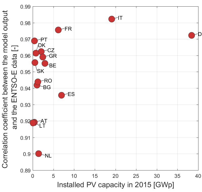
Figure 12scatter plot of the correlation coefficients between model output and ENTSO-E data against installed PV capacity for the 16 different countries.
This paper describes an innovative approach that offers a trade-off between implementation constraints and model output accuracy convenient for the goals of the C3S ECEM service and that may be used in other contexts. The validation of the model against country-aggregated production of electricity by PV plants for France and Germany shows that the model is accurate enough with a RMSE of 3–4 % of the installed capacity. In addition, the model has been further validated against solar power generation time series from 16 countries, which give correlation coefficient above 0.94 except for 4 countries (Austria, Lithuania, Netherlands, and Switzerland). The reasons for the under-average scores for these countries could unfortunately not be identified, which represents a first possible continuation of the present work. This validation revealed that the greater the installed capacity the better the performance of our model is. This finding together with the satisfying results of our performance analysis, confirm that the proposed model is well suited for our targeted applications. Indeed, the goal of the present work was not to make a perfect model for a single country but to propose a generalized approach that can be implemented in any (European) region without having to collect any specific information on the fleet of plants installed in that country. We believe an under-optimal performance is thus acceptable with respect to the gain in flexibility offered by the proposed approach.
Additional validation work would bring a better insight into the strengths and weaknesses of the proposed methodology and identify possible improvements. In addition, data on PV production is available from TSOs in many European countries and the validation may be performed for these countries thus confirming or not the performances of the model presented here. The model may be refined with respect to its parameters using more data from various countries. A possible approach to this end may consist in estimating the probability function of the regional PV model using inversion techniques, using the optimal tilt angle dependent distribution described in this paper as a first guess.
Time series of PV power generation have been calculated in the framework of the C3S ECEM service with the proposed approach using the ECEM bias-adjusted ERA interim data and future climate projections for 33 countries in a 3 h time resolution. These model output data are freely available on the demonstrator of this project: http://ecem.climate.copernicus.eu/demo
The set of adjusted reanalysis data is available on ESSD (Jones et al., 2017) and has the following DOI https://doi.org/10.5194/essd-9-471-2017. Times series of aggregated PV power generation are available at country level for all EU countries on the following ftp server ftp://ecem.climate.copernicus.eu/.
The authors declare that they have no conflict of interest.
This article is part of the special issue “17th EMS Annual Meeting: European Conference for Applied Meteorology and Climatology 2017”. It is a result of the EMS Annual Meeting: European Conference for Applied Meteorology and Climatology 2017, Dublin, Ireland, 4–8 September 2017.
The authors would like to acknowledge funding for the European Climatic
Energy Mixes (ECEM) service by the Copernicus Climate Change Service, a
programme being implemented by the European Centre for Medium-Range Weather
Forecasts (ECMWF) on behalf of the European Commission. The specific grant
number is 2015/C3S_441_Lot2_UEA.
Edited by:
Sven-Erik Gryning
Reviewed by: Sven Killinger, Hans Georg
Beyer,
and one anonymous referee
BDPV: Information from a set of ca. 20 000 PV plants installed in France, http://www.BDPV.fr, last access: February 2018.
Bright, J. M., Killinger, S., Lingfors, D., and Engerer, N. A.: Improved satellite-derived PV power nowcasting using real-time power data from reference PV systems, Sol. Energy, https://doi.org/10.1016/j.solener.2017.10.091, in press, 2017.
Jamaly, M., Bosch, J., and Kleissl, J.: Aggregate Ramp Rates Analysis of Distributed PV Systems in San Diego County, 4, 519–526, 2013.
Jerez, S., Thais, F., Tobin, I., Wild, M., Colette, A., Yiou, P., and Vautard, R.: The CLIMIX model: A tool to create and evaluate spatially-resolved scenarios of photovoltaic and wind power development, Renewable and Sustainable Energy Reviews, 42, 1–15, https://doi.org/10.1016/j.rser.2014.09.041, 2015.
Jones, P. D., Harpham, C., Troccoli, A., Gschwind, B., Ranchin, T., Wald, L., Goodess, C. M., and Dorling, S.: Using ERA-Interim reanalysis for creating datasets of energy-relevant climate variables, Earth Syst. Sci. Data, 9, 471–495, https://doi.org/10.5194/essd-9-471-2017, 2017.
Killinger, S., Guthke, P., Semmig, A., Müller, B., Wille-Haussmann, B., and Fichtner, W.: Upscaling PV Power Considering Module Orientations, IEEE J. Photovoltaics, 7, 941–944, 2017.
Lingfors, D. and Widén, J.: Development and validation of a wide-area model of hourly aggregate solar power generation, Energy, 102, 559–566, 2016.
Lorenz, E. and Heinemann, D.: Prediction of Solar Irradiance and Photovoltaic Power, in: Comprehensive Renewable Energy, 1, 239–292, https://doi.org/10.1002/pip.1224, 2012.
Marinelli, M., Maule, P., Hahmann, A. N., Gehrke, O., Nørgård, P. B., and Cutululis, N. A.: Wind and Photovoltaic Large-Scale Regional Models for Hourly Production Evaluation, IEEE Trans. Sustain. Energy, 6, 916–923, 2015.
Pierro, M., De Felice, M., Maggioni, E., Moser, D., Perotto, A., Spada, F., and Cornaro, C.: Data-driven upscaling methods for regional photovoltaic power estimation and forecast using satellite and numerical weather prediction data, Sol. Energy, 158, 1026–1038, 2017.
PV-DE: register of PV plants installed in France at the end of 2014 taken from the 4 German transmission system operators, https://www.tennettso.de/site/Transparenz/veroeffentlichungen/netzkennzahlen/tatsaechliche-und-prognostizierte-solarenergieeinspeisung, http://www.amprion.net/photovoltaikeinspeisung, http://www.50hertz.com/de/Kennzahlen/Photovoltaik, https://www.transnetbw.de/de/kennzahlen/erneuerbare-energien/fotovoltaik/ (last access: September 2016), 2014.
PV-FR: register of PV plants installed in France at the end of 2014, http://www.statistiques.developpement-durable.gouv.fr/energie-climat/r/differentes-energies-energies-renouvelables.html?tx_ttnews[tt_news]=25476&cHash=2503643552a41cb073923bec691aec02, 2014 (last access: December 2017).
Saint-Drenan, Y.-M.: A Probabilistic Approach to the Estimation of Regional Photovoltaic Power Generation using Meteorological Data, Application of the Approach to the German Case, PhD Thesis, University of Kassel, 2015.
Saint-Drenan, Y.-M., Bofinger, S., Fritz, R., Vogt, S., Good, G.-H., and Dobschinski, J.: An empirical approach to parameterizing photovoltaic plants for power forecasting and simulation, Sol. Energy, 120, 479–493, https://doi.org/10.1016/j.solener.2015.07.024, 2015.
Saint-Drenan, Y.-M., Good, G.-H., Braun, M., and Freisinger, T.: Analysis of the uncertainty in the estimates of regional PV power generation evaluated with the upscaling method, Sol. Energy, 135, 536–550, https://doi.org/10.1016/j.solener.2016.05.052, 2016.
Saint-Drenan, Y.-M., Good, G., and Braun M.: A probabilistic approach to the estimation of regional photovoltaic power production, Sol. Energy, 147, 247–276, https://doi.org/10.1016/j.solener.2017.03.007, 2017.
Schierenbeck, S., Graeber, D., Semmig, A., and Weber, A.: Ein distanzbasiertes Hochrechnungsverfahren für die Einspeisung aus Photovoltaik, Energiewirtschaftliche Tagesfragen, 2010.
Schubert, G.: Modeling hourly electricity generation from PV and wind plants in Europe, 9th Int. Conf. Eur. Energy Mark. EEM, 12, 1–7, 2012.
Shaker, H., Zareipour, H., and Wood, D.: A data-driven approach for estimating the power generation of invisible solar sites, IEEE T. Smart Grid, 99, https://doi.org/10.1109/TSG.2015.2502140, 2015.
Shaker, H., Zareipour, H., and Wood, D.: Estimating power generation of invisible solar sites using publicly available data, IEEE T. Smart Grid, 99, https://doi.org/10.1109/TSG.2016.2533164, 2016.
Troccoli, A., Goodess, C., Jones, P., Penny, L., Dorling, S., Harpham, C., Dubus, L., Parey, S., Claudel, S., Khong, D.-H., Bett, P., Thornton, H., Ranchin, T., Wald, L., Saint-Drenan, Y.-M., De Felice, M., Brayshaw, D., Suckling, E., Percy, B., and Blower, J.: The Copernicus Climate Change Service “European Climatic Energy Mixes”, EMS Annual Meeting 2017, Dublin, Ireland, 4–8 September 2017, Abstract EMS2017-824, 2017.