 | 08 Jun 2018
Bias adjustment for threshold-based climate indicators
Christoph Menz
Arne Spekat
A method is presented which applies bias adjustments to climate indicators that are based on fixed thresholds, e.g., the number of hot days with the maximum temperature exceeding 30 ∘C or the number of days with heavy precipitation in exceedance of 20 mm rainfall. The bias adjustment first identifies the percentile of the required threshold value in reference climate data. Then it computes the value of this percentile for the individual historical climate model simulations – here an ensembles of EURO-CORDEX model runs, including dynamical and statistical models. Finally, the climate indicator is re-calculated for each model. The method is applied to climate projections as well, giving further insight into the projected development of the ensemble for extreme conditions. It is assessed that communication to the public and decision makers is improved by expressing these changes in extremes based on absolute values.


1.1 Context
The majority of climate models – global climate models as well as regional climate models – exhibit systematic differences between the observed current climate (e.g. in the reference period 1971–2000) and the simulated climate. The technical term for this deviation is bias. Statistical regional climate models, also called Empirical Statistical Downscaling Models (ESDs) typically have a smaller bias than dynamical models, also called Regional Climate Models (RCMs), since they are based on observation data. Climate and climate impact research relies on simulations with no considerable bias in order to be applicable for future time frames (Gobiet et al., 2015). Thus, it is self-evident to reduce it by a bias adjustment, as stated in Christensen et al. (2008).
Most bias adjustment approaches are based on the stationarity assumption of the bias (Grillakis et al., 2016), i.e., they assume that the model bias is not changing in time. This underlying assumption needs to be taken into account when analysing bias adjusted model results or using them in impact assessments, since it can distort the time series or add an artificial component to the modeled climate change (Chen et al., 2015; Maraun, 2012). The standard procedure of bias adjustment is to apply it to individual parameters of a climate simulation, e.g., precipitation or near-surface temperature. However, interrelations between different modelled variables (e.g., between temperature and humidity or between precipitation, soil water contents and air temperature) are not taken into account. This assumption ignores the reality of a fully coupled climate system and can potential result in spurious model fields, rendered by the bias adjustment (Ehret et al., 2012; Rocheta et al., 2014). It could be shown, that this deficiency have a significant impact on the adjusted fields and impair the usage of the adjusted fields (Chun et al., 2014; Muerth et al., 2013; White and Toumi, 2013) introducing artificial errors. However recently more and more bias adjustment approaches emerge, taking care of the multivariate structure of the system under adjustment (Cannon, 2016; Piani and Haerter, 2012; Vrac and Friederichs, 2015). Advantages and limitations of bias adjustment methods are summarized in Maraun (2016).
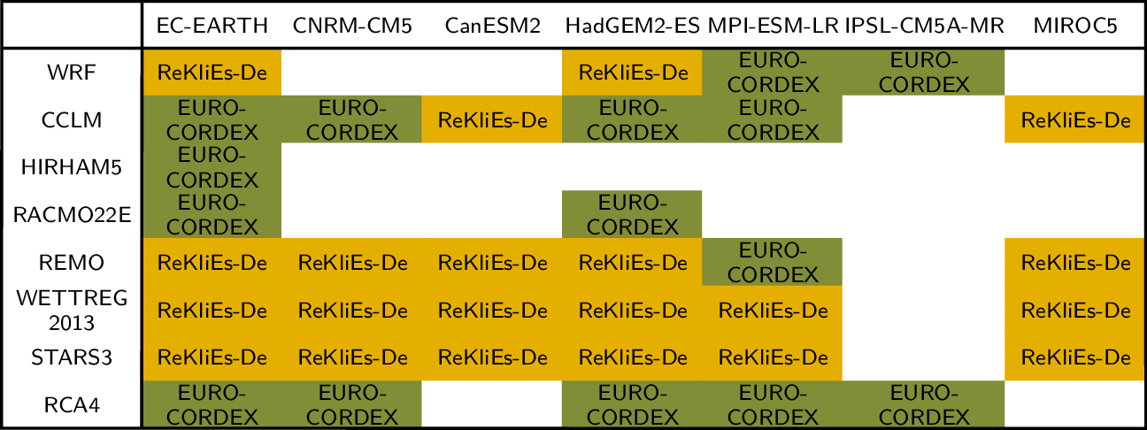
Table 1Pooled EURO-CORDEX simulations (green) and added simulations by ReKliEs-De (orange).
The stationarity assumption and univariability of most bias adjustment approaches used to-date can yield to artificial errors in model fields that, in turn, could influence decisions by end users. It is therefore important to communicate the side effects of applying a bias adjustment. The Project ReKliEs-De (Regionale Klimaprojektionen Ensemble für Deutschland; Ensemble of regional climate projection for Germany) not only had a focus on contributing to EURO-CORDEX by producing runs of dynamical and statistical climate models (Hübener et al., 2017a); it also had a focus on addressing end user needs (Hübener et al., 2017b). ReKliEs-De produced geographical distributions of 24 climate indicators, mostly temperature- and precipitation-based1 This posed a new challenge since so far bias adjustments were devised to be applied to climate parameters but not to indicators.
Within ReKliEs-De we use three different approaches to deal with model inherent biases. We tried to use bias-independent indicators as much as possible to circumvent potential deficiencies introduced by the model bias. In all other cases we applied two different types of bias adjustment. Indicators based on fixed thresholds were adjusted using the method described in this article. All other indicators were adjusted using a classical bias adjustment approach. Both bias adjustment approaches used in ReKliEs-De were applied to single variables (ignoring covariables) and assume bias stationarity.
1.1.1 Bias-independent indicators
Whenever the indicators are based on a relative measure, such as a quantile, they are bias-free by definition. Examples for this type of indicators are tx90p (number of days above the 90th percentile of daily maximum temperature), tx10p (number of days below the 10th percentile of daily maximum temperature), wsdi (warm spell duration index) csdi (cold spell duration index), r95ptot (precipitation amount above the 95th percentile) and r99ptot (precipitation amount above the 99th percentile). The threshold itself is subject to the individual model's bias.
1.1.2 Indicators based on fixed thresholds
Numerous climate indicators are computed using prescribed thresholds. The indicator su30, for example, counts the days on which the maximum temperature exceeds a threshold of 30 ∘C. However, this threshold is influenced by the model bias. The bias adjustment is then performed by determining the percentile belonging to this threshold from climate reference data and subsequently modifying the threshold itself according to that percentile. Then the procedure of determining the day count is repeated using the modified threshold (Hoffmann et al., 2017) which will lead to similar values as the reference. The bulk of this paper will deal with this threshold-modifying approach.
1.1.3 Classical bias adjustment approaches
A bias adjustment of this type directly changes simulated variables using a set of prescribed rules to adapt the simulations to fit the reference data. Those rules are devised in view of the target variable, e.g., the monthly mean precipitation or the distribution of daily precipitation intensities. Moreover, there is a dependency upon the reference dataset used. A rather simple bias adjustment would consist of a linear shift of the data (adding to or subtracting from the values). More sophisticated bias adjustment methods result in complex effects on climate change signals. Two methods are frequently applied: (i) Local Intensity Scaling (LOCI) described, e.g., in Schmidli et al. (2006) and (ii) Analytical Quantile Mapping (AQM), described, e.g., in Sun et al. (2011) or Themeßl et al. (2012). An overview of these and further bias adjustment methods can be found in Fang et al. (2015).
1.2 Structure of the paper
The paper continues with a summary description of the ReKliEs-De simulation matrix (GCM-RCM combination) as the basis for the climate extreme assessment by calculating threshold-based climate indicators (Sect. 2). In order to minimize the existing bias of the raw data against observations we introduce a new approach which defines a model-specific adjusted threshold without touching or manipulating the raw data (Sect. 3). For the climate indicators su30 and r20mm all patterns in historical simulations with and without adjusted threshold are compared and discussed (Sect. 4). Comparisons to other approaches are summarized in the end (Sect. 5).
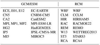
The ensemble contains regional climate model simulations of the ReKliEs-De and EURO-CORDEX projects (Table 1). Besides state-of-the-art dynamical regional downscaling models (RCMs) also empirical-statistical downscaling models (ESDs) were used. The total ensemble consists of 6 different RCMs (WRF, CCLM, HIRHAM5, RACMO22E, REMO and RCA4) and 2 ESDs (WETTREG2013 and STARS3) driven by 7 different Global Climate Models (EC-EARTH, CNRM-CM5, CanESM2, HadGEM2-ES, MPI-ESM-LR, IPSL-CM5A-MR, MIROC5). Table 2 displays all combinations of RCMs and GCMs that were analyzed and allocates them to their respective project. Within ReKliEs-De, GCMs were selected with the aim to cover the spread of anticipated near-to-midterm (until 2100) temperature and precipitation changes in the area Germany drawn from all available CMIP5 models.
Following the CORDEX-EUR11 protocol all RCM simulations cover the European continent on a 0.11∘ (approx. 12 km) grid. The ESD simulations use the same grid, but covering just the Central European part of the domain, due to their inherent methodological restrictions. Our analysis encompasses the historical and RCP8.5 model runs (Jacob et al., 2013) for a total period of 1971–2100.
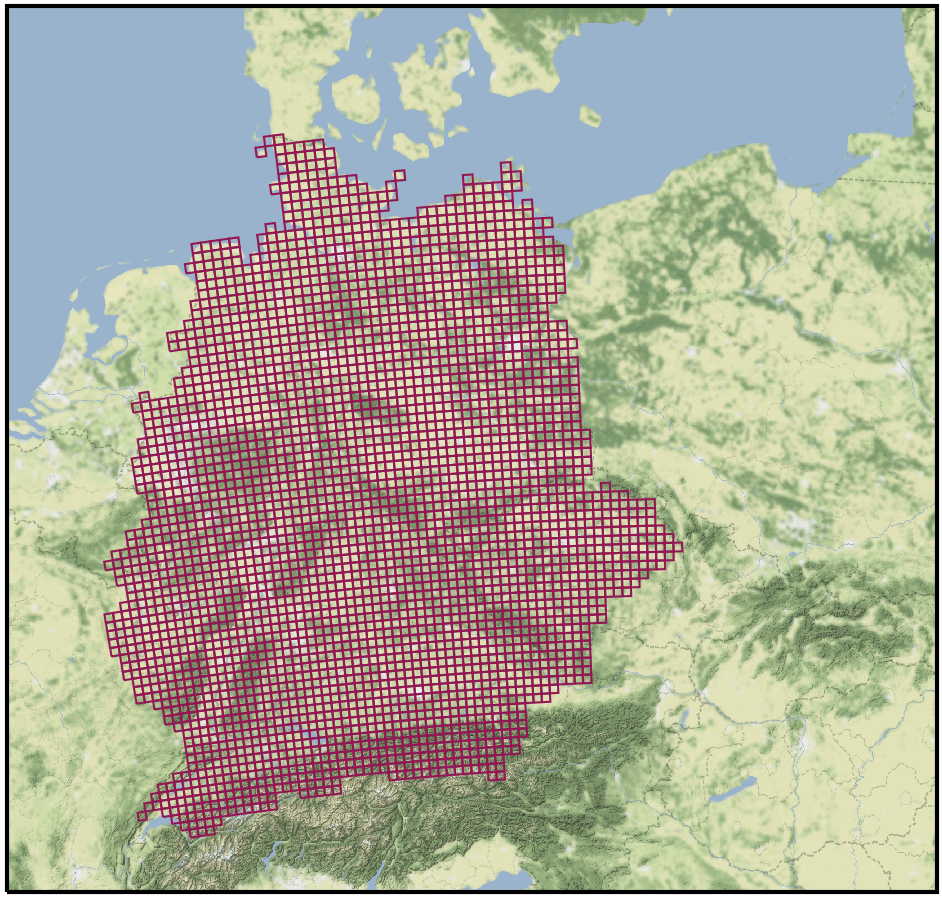
Figure 1EURO-CORDEX grid cells used for the analyses – the ReKliEs-De area. It includes Germany and several catchments of rivers discharging into Germany.
In some cases, specific GCM and RCM versions are used for different combinations. See Hübener et al. (2017a) for a detailed model matrix, which specifies the model names and versions.
We focus our analysis on a Central European domain according to the ReKliEs-De project definitions. This domain is defined by all grid boxes over land areas that belong to river catchments discharging into German territory. The eight main river catchments are Danube, Elbe, Ems, Main, Mosel, Neckar, Rhine and Weser. The resulting mask covers mainly Germany and parts of the Czech Republic as well as parts of the alpine region. Figure 1 shows a map of all grid boxes considered in our analysis.
Within the ReKliEs-De project 24 standard climate indicators were calculated, including those which are used in this study:
-
tasmax [∘C]: daily maximum near surface (2 m) air temperature;
-
pr [mm]: daily sum of precipitation;
-
su30 [days]: number of hot days (tasmax >30 ∘C);
-
r20mm [days]: number of days with very heavy precipitation (pr >20 mm).
The quality of the bias adjustment depends on the quality of the reference data set. The reference dataset used in this study is based on a combination of two data sources interpolated onto the same grid as the model data (the CORDEX-EUR11 grid): (1) the climate station network provided by the German Weather Service (DWD) and (2) the European gridded dataset EOBS-0.22deg-rot-v15.0 (Haylock et al., 2008). The interpolation is based on Rudolf et al. (1992) which utilizes a distance and directional weight. Hence two stations lying in the same direction of the grid point (e.g. both north of the grid point) will have a lower weight than two stations lying in opposite directions (e.g. north and south of the grid point). As for the reference orography, we selected an orography based on SRTMv3 which was bilinearly interpolated onto the 0.11∘ CORDEX-EUR11 grid. For the interpolation of the temperature fields a constant lapse rate of 0.65 K∕100 m was applied. We used no height adjustment for the precipitation fields.
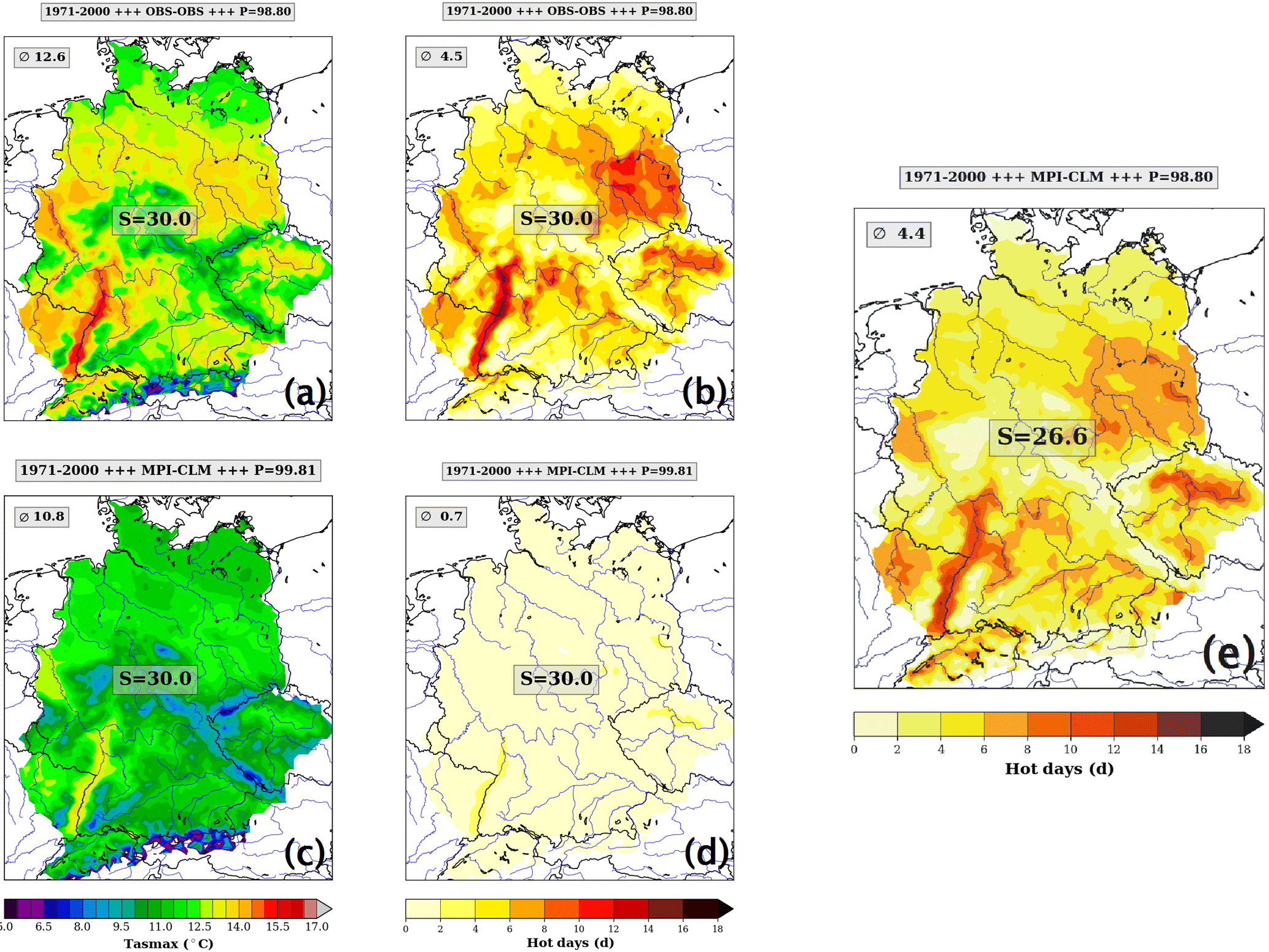
Figure 2Work flow of the threshold adjustment approach, indicated by (a)–(d). First row: tasmax (OBS) → su30 (OBS). Second row: → tasmax (RCM) → su30 (RCM). Larger graph (e): Resulting map for su26.6 (RCM). The box in the upper left corner of each subfigure indicates the areal average (∅) for the ReKliEs-De domain. The box in the center of each subfigure shows the temperature threshold [∘C] used to determine the number of hot days. The percentile of the temperature threshold is given in the right-hand side of the bar over the figure. This bar also shows on its left-hand side which period is used and the text in its center denotes if observations (OBS) or a GCM-RCM combination (in this example: MPI-CLM) is used.
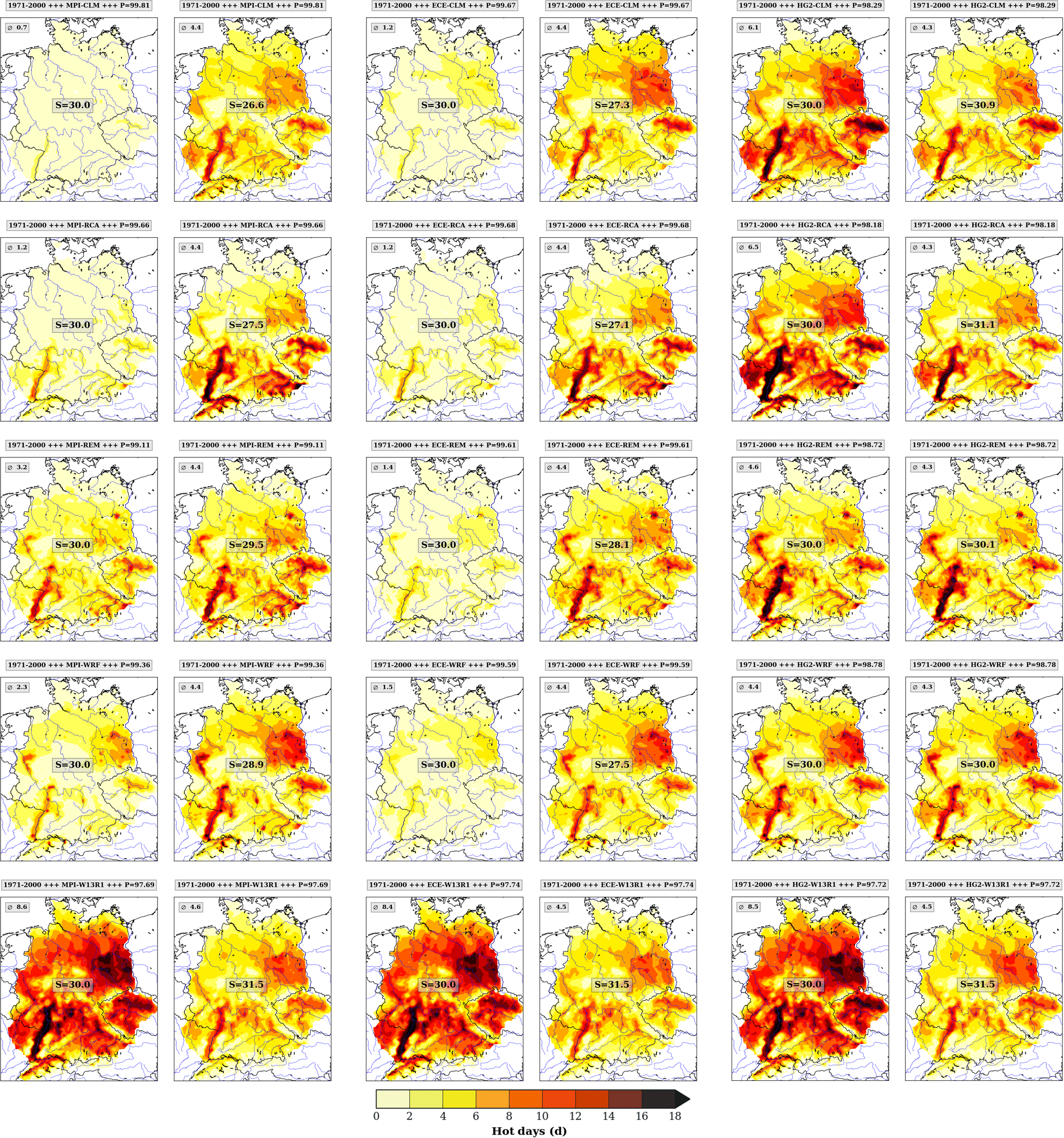
Figure 3Comparison of su30 (hot days with a maximum above 30 ∘C) regionalizations using 20C/historical runs data from the period 1971–2000. The forcing GCMs are arranged in columns and the RCMs in rows. Each row contains three pairs of maps for the three GCMs used, showing su30 without (left) and with (right) bias adjustment.
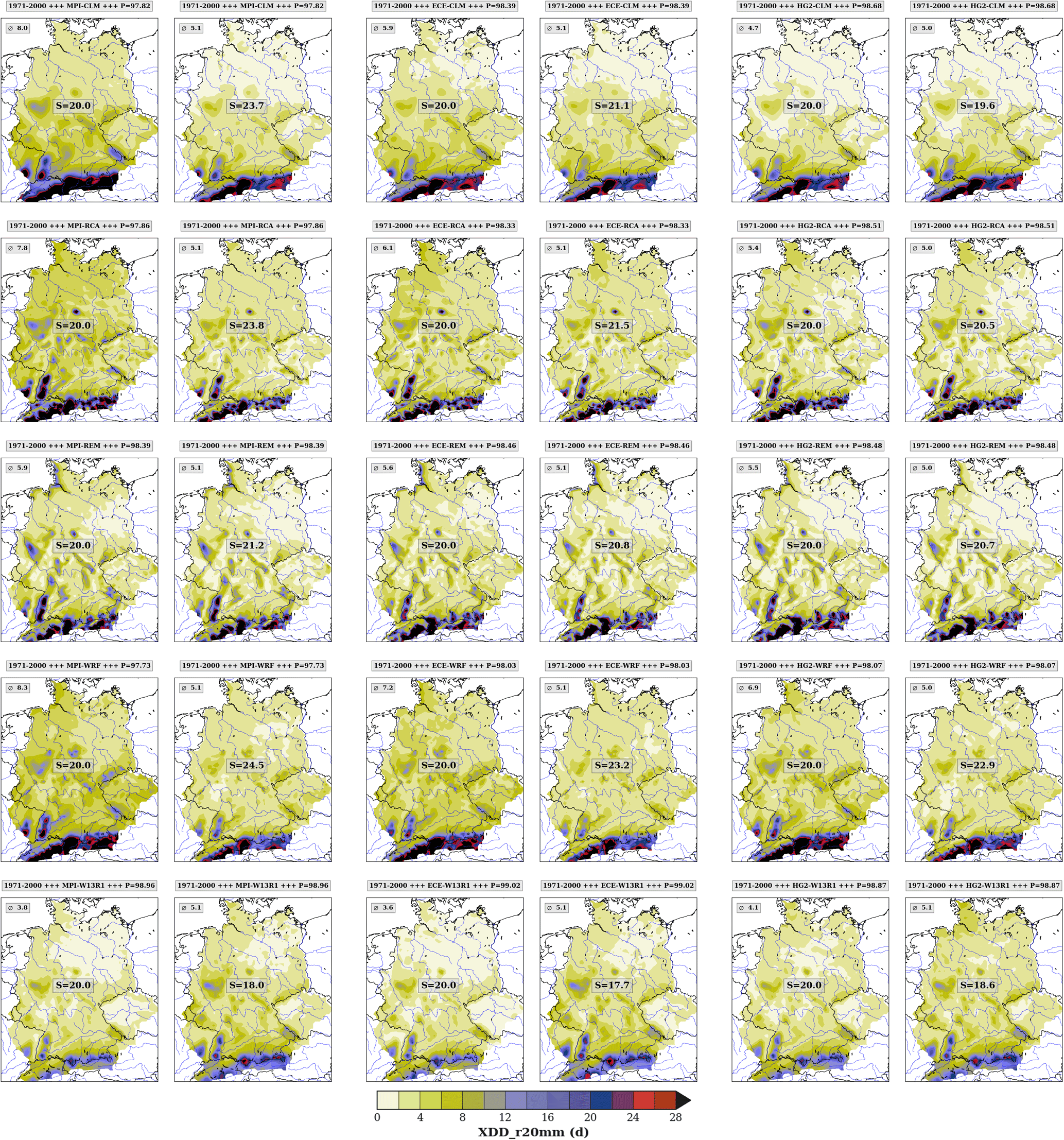
Figure 4As in Fig. 3 but for r20mm (number of days with heavy precipitation of 20 mm or more).
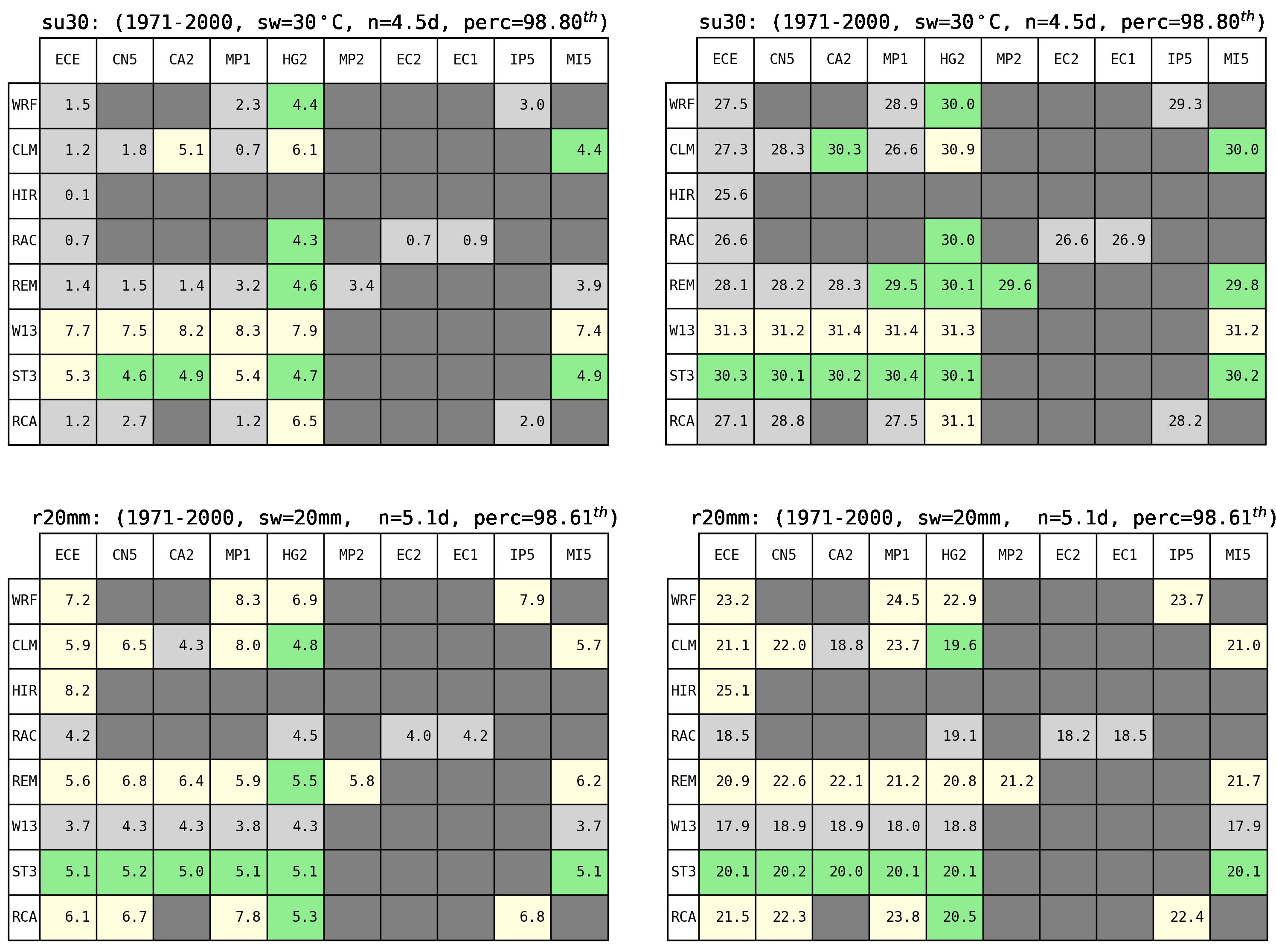
Table 3Simulations of two threshold-based climate indicators (top: su30; bottom: r20mm) within the ReKliEs-De region and the period 1971–2000. Columns of every table – forcing global models. Lines of every table – RCMs or ESDs. Pairs of tables are displayed, left – simulated values, right – adjusted thresholds for the indicator. Light grey boxes – value is below the climatological average. Light yellow boxes – value is above the climatological average. Green boxes – average is met within a margin of 0.5 units (top left and bottom left: days, top right: ∘C; bottom right: mm). Numbers above each table denote the threshold value (sw), the frequency of occurrence in days (n) and the percentile of the threshold (perc) computed from climate averages.
The method was designed to adjust the bias for climate extremes, e.g. the number of hot days (su30) and the number of very wet days (r20mm) in regional climate model simulations. It is important to note that it had been a priority not to alter the simulation data, themselves. A basic assumption is that climate indicators using fixed thresholds must be applicable for the entire area of interest, encompassing mountainous as well as lowland regions. The underlying idea is to identify thresholds in the simulations of the reference period (1971–2000) which are specific to the individual GCM-RCM combinations and compare them to the defined fixed thresholds in the observed climate for the same period.
An overview of the work flow for the temperature indicator su30 is given in Fig. 2. The algorithm is as follows: We start by calculating the percentile values Psu30 and Pr20mm in the gridded daily observation data (1971–2000). Subsequently, the historical simulations for the period 1971–2000 by the GCM-RCM combinations are used to determine the values related to the percentiles calculated in the observation data. This is performed for every GCM-RCM combination. In most cases the resulting thresholds are exhibiting a bias, i.e., the thresholds are not matching those from the observation data, with model-specific deviations towards higher or lower thresholds. Therefore the thresholds need to be adjusted. The indicators for the period 1971–2000 are calculated a second time, using the bias-adjusted thresholds instead of the fixed thresholds (30 ∘C for su30 or 20 mm for r20mm, respectively). Their values are then very close to the observations, meeting the aim of the bias adjustment. For intercomparison purposes, threshold matrices are given in Table 3 for the model ensemble with su30 in the upper and r20mm in the lower row.
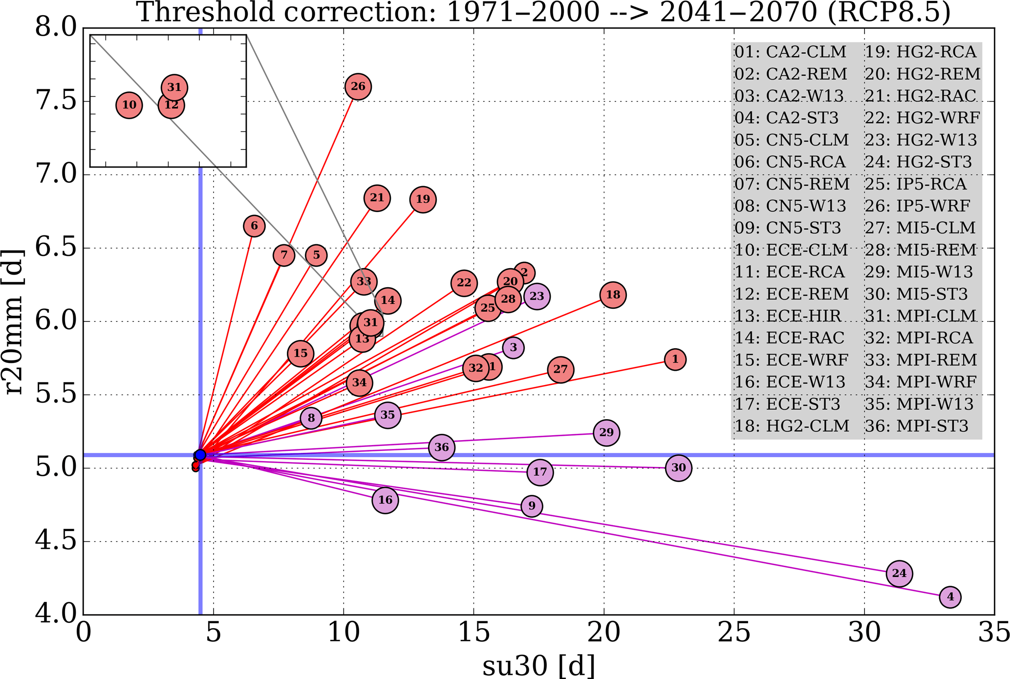
Figure 5Scatterplot of the projected number of hot days (su30) and very wet days (r20mm) using threshold adjusted RCM (red) and ESD (magenta) simulations until 2041–2070 (RCP8.5). The simulations are numbered for reference in the right-hand tabulation. The window in the top left corner enlarges the a segment of the graph near the label for model chain 31 (MPI-CLM) where several labels are overlapping. Thick blue lines mark the baseline period (1971–2000) conditions for su30 and r20mm.
To further illustrate the steps of the method, details from an analysis using a simulation of the global model MPI-ESM r1i1p1 (MP1) forcing the regional model CCLM (CLM) are presented here for su30. Within the reference period (1971–2000) and for the ReKliEs-De domain, the simulated long-term annual mean of tasmax is 1.8 K lower than the observed annual mean of the maximum temperature, cf. the boxes in the upper left part of Fig. 2c and a. As a consequence of the simulated lower mean of the maximum temperature, the number of hot days (su30), averaged over the whole domain is much lower in the climate simulation by MP1–CLM (0.7 days, Fig. 2d) than in the observed climate (4.5 days, Fig. 2b). According to our method, we adjust the threshold of 30 ∘C, so that the count of hot days approaches the observed 4.5 days. This is achieved by using all grid points of the ReKliEs-De domain from the years 1971–2000 of the gridded observation data to calculate the percentile which belongs to the fixed threshold of 30 ∘C. For this paricular threshold, a percentile of 98.80 is determined. In the next step the tasmax value belonging to the percentile of 98.80 is identified in the MP1–CLM simulation for the period 1971–2000 and all grid points of the ReKliEs-De domain. It is found to be 26.6 ∘C. This constitutes the new bias adjusted threshold for the recalculation of su30 for MP1–CLM which turns from a su30 to a su26.6. As Fig. 2e shows, the resulting area average for the indicator su30 simulated by the bias-adjusted MP1–CLM (4.4 days) is very close to that from observed data in Fig. 2b. Moreover, the spatial patterns of modelled and observed data have a close resemblance, too (cf. Fig. 2b and e).
In the frame of the ReKliEs-De project, further climate indicators based on fixed thresholds (e.g., id, su, r10mm, gsl) are subjected to the same bias adjustment process. With the bias adjustment for those indicators established, the model specific-thresholds are used to determine the indicators in model projections for the entire 21st century.
The method, described in Sect. 3 has been applied to the entire ReKliEs-De ensemble in order to assess climate extremes and their climate sensitivity. In the following paragraphs we discuss the individual patterns (maps) for su30 and r20mm with and without threshold adjustment. We also discuss the underlying threshold matrix and present the results of future projections.
The left-hand tables in Table 3 show the simulated su30 and r20mm values averaged over the RekliEs-De domain for the historical period (1971–2000) without threshold adjustment. The colors indicate the direction of the model bias, negative (light grey) and positive (light yellow) compared to the climate indicators derived from observations. Similar values are colored in light green. Since most of the RCMs have a cold bias (Hübener et al., 2017b), the su30 numbers are frequently underestimated, e.g., for EC-EARTH forcing REMO (ECE–REM), 1.4 occurrences of su30 are computed for the ReKliEs-De area in the simulation of the period 1971–2000, whereas the measurements yield a count of 4.5 days. There is a reversed situation for r20mm. Here, the RCMs frequently overestimate the mean precipitation patterns for the ReKliEs-De domain and also the r20mm indicator.
The right-hand tables of Table 3 depict the adjusted thresholds for su30 and r20mm, respectively. They range from 25.6 ∘C (ECE–HIR) to 31.4 ∘C (CA2–W13 and MP1–W13) for su30 and from 25.1 mm (ECE–HIR) to 17.9 mm (ECE–W13 and MI5–W13) for r20mm. Applying these threshold adjustments, the values of su30 and r20mm amount to nearly 4.5 and 5.1 days, respectively, for all ensemble members.
The resulting patterns for the 1971–2000 period with and without adjusted thresholds are shown in Fig. 3 (su30) and Fig. 4 (r20mm) for three GCMs (MP1, ECE and HG2). After adjustment, all patterns show similar regional characteristics with just minor differences. Without threshold adjustments most of the model members underestimate the averaged number of su30 by almost 4 days (e.g. MPI-CLM, MPI-RCA, ECE-CLM, ECE-RCA). Simulations with HG2-REM and HG2-WRF, on the other hand, exhibit a rather close match to the climate conditions. The comparison of the r20mm patterns with and without threshold adjustments reveals positive bias up to about 3 days (e.g. MPI–CLM and MPI–WRF).
In order to assess the future development of su30 and r20mm for the ReKliEs-De domain the climate indicators were calculated for every model member in an RCP8.5 simulation by using the adjusted threshold, respectively. Figure 5 depicts the changes for each model combination. It shows the climate signals between the periods 2041–2070 and 1971–2000. The RCMs are represented in Fig. 5 by red lines and the ESDs by magenta lines. The observed state for the baseline period is indicated by thick blue lines. The conditions of the period 1971–2000 for all ensemble members after bias adjustment are gathered at the 4.5;5.1 days point, i.e., they closely approximate the observations. Since the signals are determined from projections using an RCP8.5 scenario it can be inferred that without climate protection the number of hot days (su30) will change until 2041–2070 between 8.8 and 21.5 days – the range is determined using the 10th and the 90th percentile of the ensemble. This behaviour is corroborated by all models. For r20mm two modelling families can be distinguished: RCMs and ESDs. They exhibit different trend directions with a decrease in r20mm for the ESDs and a clear increase for the RCMs. Model combinations which simulate a strong increase of su30 show a smaller increase of r20mm, and vice versa. All RCMs in the ReKliEs-De ensemble simulate an increase in the number of extreme weather days (su30 and r20mm).
Simulations of regional climate models suffer from model bias and users should be aware of this fact. The simulated climate average for the historical period may be 1–2 K below the observed average whereas, e.g., the number of hot days (su30) is clearly lower. This also strongly varies depending on the reference dataset used.
By the approach described in this paper we adjusted the point of view for each climate indicator in order to arrive at a similar mean level. This enhances the comparability of regional features and climate sensitivity considerations.
This approach does not aim at replacing established bias adjustments as an important intermediate stage for regional impact assessments. Yet, it improves the qualitative evaluation of features in regional climate ensembles without injecting too much complexity.
Such an application has its spatial limitations. The ReKliEs-De area is rather large and stretches the concept of obtaining feasible area statistics for climate indicators. However, the method could also be applied to single grid boxes or sub-domains. In that case the area must be of sufficient size and appropriate location, so that there are enough events defined by the threshold in the model simulations and the observations. In addition, border effects might occur, once the area in which the amount of threshold correction is determined differs from that in which the threshold correction is applied. It should be added that the quality of the results highly depends on the quality of the observation data. A final remark: An investigation to what extent the derived adjusted threshold matrix can be transferred to other variables would have been beyond the scope of this study.
Data of regionalizations was provided by ReKliEs-De model runs, augmented by other EURO-CORDEX runs, available from the World Data Center for Climate, Hamburg, Germany, through their website at http://cera-www.dkrz.de (WDC Climate, 2018). Access to the ReKliEs-De data is provided through http://reklies.hlnug.de/startseite/ (HLNUG, 2018). Please select the last entry on that web page and subsequently scroll to the table at the end of this web document.
PH has developed the methodology. PH and CM devised the computational algorithms and performed the computations. PH and AS produced graphic and tabular material. AS and PH compiled the paper, all authors discussed and corrected the paper. All authors read and approved the final manuscript.
The authors declare that they have no conflict of interest.
This article is part of the special issue “17th EMS Annual Meeting: European Conference for Applied Meteorology and Climatology 2017”. It is a result of the EMS Annual Meeting: European Conference for Applied Meteorology and Climatology 2017, Dublin, Ireland, 4–8 September 2017.
The project ReKliEs-De was carried out under grant 01LK1401 of the German
Ministry of Education and Research (BMBF).
The
article processing charges for this open-access
publication
were covered by the Potsdam Institute
for Climate Impact
Research (PIK).
Edited by: Fulvio Stel
Reviewed by: Teodoro Georgiadis, Massimo Enrico Ferrario,
and one anonymous referee
Cannon, A.: Multivariate Bias Correction of Climate Model Output: Matching Marginal Distributions and Intervariable Dependence Structure, J. Climate, 29, 7045–7064, https://doi.org/10.1175/JCLI-D-15-0679.1, 2016. a
Chen, J., Brissette, F., and Lucas-Picher, P.: Assessing the limits of bias-correcting climate model outputs for climate change impact studies, J. Geophys. Res.-Atmos., 120, 1123–136, https://doi.org/10.1002/2014JD022635, 2015. a
Christensen, J., Boberg, F., Christensen, O., and Lucas-Picher, P.: On the need for bias correction of regional climate change projections of temperature and precipitation, Geophys. Res. Lett., 35, L20709, https://doi.org/10.1029/2008GL035694, 2008. a
Chun, K., Wheater, H., and Barr, A.: A multivariate comparison of the BERMS flux-tower climate observations and Canadian Coupled Global Climate Model (CGCM3) outputs, J. Hydrol., 519, 1537–1550, https://doi.org/10.1016/j.jhydrol.2014.08.059, 2014. a
Ehret, U., Zehe, E., Wulfmeyer, V., Warrach-Sagi, K., and Liebert, J.: HESS Opinions “Should we apply bias correction to global and regional climate model data?”, Hydrol. Earth Syst. Sci., 16, 3391–3404, https://doi.org/10.5194/hess-16-3391-2012, 2012. a
Fang, G. H., Yang, J., Chen, Y. N., and Zammit, C.: Comparing bias correction methods in downscaling meteorological variables for a hydrologic impact study in an arid area in China, Hydrol. Earth Syst. Sci., 19, 2547–2559, https://doi.org/10.5194/hess-19-2547-2015, 2015. a
Gobiet, A., Suklitsch, M., and Heinrich, G.: The effect of empirical-statistical correction of intensity-dependent model errors on the temperature climate change signal, Hydrol. Earth Syst. Sci., 19, 4055–4066, https://doi.org/10.5194/hess-19-4055-2015, 2015. a
Grillakis, M. G., Koutroulis, A. G., Daliakopoulos, I. N., and Tsanis, I. K.: Addressing the assumption of stationarityin statistical bias correction of temperature, Earth Syst. Dynam. Discuss., https://doi.org/10.5194/esd-2016-52, 2016. a
Haylock, M. R., Hofstra, N., Klein Tank, A. M. G., Klok, E. J., Jones, P. D., and New, M.: A European daily high-resolution gridded data set of surface temperature and precipitation for 1950–2006, J. Geophys. Res., 113, D20119, https://doi.org/10.1029/2008JD010201, 2008. a
HLNUG (Hessisches Landesamt für Naturschutz, Umwelt und Geologie): Regionale Klimaprojektionen Ensemble für Deutschland (ReKliEs-De), available at: http://reklies.hlnug.de/startseite/, last access: 6 June 2018.
Hoffmann, P., Menz, C., and Spekat, A.: Threshold Correction of Regional Climate Model Ensembles for Climate – Extreme Assessments on the Country Level, in: 17th Annual Meeting of the European Meteorological Sociey, Dublin, 4–8 September 2017, Session UP1.3, Presentation P93, 2017. a
Hübener, H., Bülow, K., Fooken, C., Früh, B., Hoffmann, P., Höpp, S., Keuler, K., Menz, C., Mohr, V., K.Radtke, Ramthun, H., Spekat, A., Steger, C., Toussaint, F., Warrach-Sagi, K., and Woldt, M.: ReKliEs-De Ergebnisbericht, Tech. rep., Hessian Agency for Nature, Environment and Geology (HLNUG), 2017a (in German). a, b
Hübener, H., Spekat, A., Bülow, K., Früh, B., Keuler, K., Menz, C., K.Radtke, Ramthun, H., Rathmann, T., Steger, C., Toussaint, F., and Warrach-Sagi, K.: ReKliEs-De Nutzerhandbuch, Tech. rep., Hessian Agency for Nature, Environment and Geology (HLNUG), 2017b (in German). a, b
Jacob, D., Petersen, J., Eggert, B., Alias, A., Bøssing Christensen, O., Bouwer, L., Braun, A., Colette, A., Déqué, M., Georgievski, G., Georgopoulou, E., Gobiet, A., Menut, L., Nikulin, G., Haensler, A., Hempelmann, N., Jones, C., Keuler, K., Kovats, S., Kröner, N., Kotlarski, S., Kriegsmann, A., Martin, E., van Meijgaard, E., Moseley, C., Pfeifer, S., Preuschmann, S., Radermacher, C., Radtke, K., Rechid, D., Rounsevell, M., Samuelsson, P., Somot, S., Soussana, J.-F., Teichmann, C., Valentini, R., Vautard, R., Weber, B., and Yiou, P.: EURO-CORDEX: new high-resolution climate change projections for European impact research, Reg. Env. Change, 14, 563–578, https://doi.org/10.1007/s10113-013-0499-2, 2013. a
Maraun, D.: Nonstationarities of regional climate model biases in European seasonal mean temperature and precipitation sums, Geophys. Res. Lett., 39, L06706, https://doi.org/10.1029/2012GL051210, 2012. a
Maraun, D.: Bias Correcting Climate Change Simulations – a Critical Review, Curr. Clim. Change Rep., 2, 211–220, https://doi.org/10.1007/s40641-016-0050-x, 2016. a
Muerth, M. J., Gauvin St-Denis, B., Ricard, S., Velázquez, J. A., Schmid, J., Minville, M., Caya, D., Chaumont, D., Ludwig, R., and Turcotte, R.: On the need for bias correction in regional climate scenarios to assess climate change impacts on river runoff, Hydrol. Earth Syst. Sci., 17, 1189–1204, https://doi.org/10.5194/hess-17-1189-2013, 2013. a
Piani, C. and Haerter, J. O.: Two dimensional bias correction of temperature and precipitation copulas in climate models, Geophys. Res. Lett., 39, L20401, https://doi.org/10.1029/2012GL053839, 2012. a
Rocheta, E., Evans, J., and Sharma, A.: Assessing atmospheric bias correction for dynamical consistency using potential vorticity, Env. Res. Lett., 9, 124010, https://doi.org/10.1088/1748-9326/9/12/124010, 2014. a
Rudolf, B., Hauschild, M., Reiss, M., and Schneider, U.: Die Berechnung der Gebietsniederschläge im 2.5∘-Raster durch ein objektives Analyseverfahren, Meteorol. Z., 1, 32–50, 1992. a
Schmidli, J., Frei, C., and Vidale, P.: Downscaling from GC precipitation: A benchmark for dynamical and statistical downscaling methods, Int. J. Climatol., 26, 679–689, https://doi.org/10.1002/joc.1287, 2006. a
Sun, F., Roderick, M., Lim, W., and Farquhar, G.: Hydroclimatic projections for the Murray-Darling Basin based on an ensemble derived from Intergovernmental Panel on Climate Change AR4 climate models, Water Res. Res., 47, W00G02, https://doi.org/10.1029/2010wr009829, 2011. a
Themeßl, M., Gobiet, A., and Heinrich, G.: Empirical-statistical downscaling and error correction of regional climate models and its impact on the climate change signal, Clim. Change, 112, 449–468, 2012. a
Vrac, M. and Friederichs, P.: Multivariate-Intervariable, Spatial, and Temporal-Bias Correction, J. Climate, 28, 218–237, https://doi.org/10.1175/JCLI-D-14-00059.1, 2015. a
WDC Climate (World Data Center for Climate): DKRZ long term archive, available at: https://cera-www.dkrz.de, last access: 6 June 2018.
White, R. H. and Toumi, R.: The limitations of bias correcting regional climate model inputs, Geophys. Res. Lett., 40, 2907–2912, https://doi.org/10.1002/grl.50612, 2013. a
For nomenclature and definitions of climate indicators, see http://etccdi.pacificclimate.org/list_27_indices.shtml, last access: 4 June 2018.